Quick Start
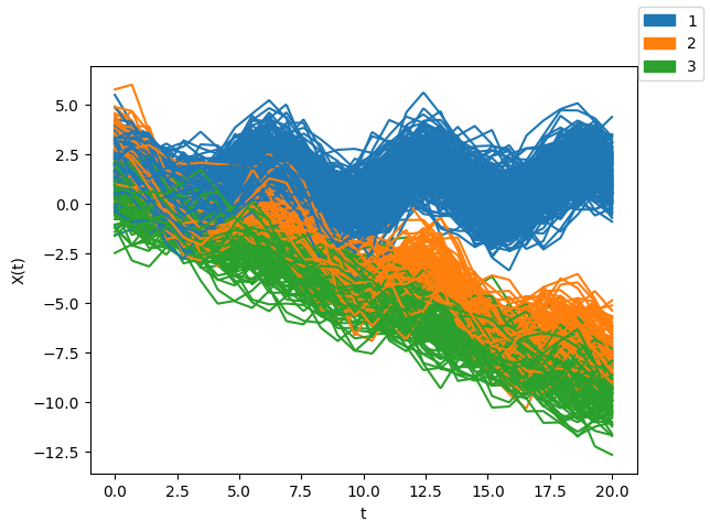
This guide shows how to use the package with simulated data. We’ll generate synthetic functional data from a mixture of Gaussian processes and prepare it for analysis:
import numpy as np
import matplotlib.pyplot as plt
import scipy
import skfda

def exponentiated_quadratic(xa, xb):
   sq_norm = -0.5 * scipy.spatial.distance.cdist(xa, xb, 'sqeuclidean')
   return np.exp(sq_norm)

def get_data():
   nb_of_samples = 30
   t = np.expand_dims(np.linspace(0, 20, nb_of_samples), 1)
   Σ = exponentiated_quadratic(t, t)

   mean_curve = np.zeros((3, len(t)))
   mean_curve[0] = np.reshape(np.cos(t), (nb_of_samples))
   mean_curve[1] = np.reshape(np.cos(t) -0.5*t, (nb_of_samples))
   mean_curve[2] = np.reshape(-0.5*t + 0.5, (nb_of_samples))

   mixture_k = [1/2, 1/4, 1/4]
   n = 500
   Y = np.zeros((n, len(t)))
   simulation_label = np.zeros(n)

   for i in range(n):
      r = np.random.rand()
      if r <= mixture_k[0]:
            ys = 1 + np.random.multivariate_normal(mean= mean_curve[0], cov=Σ, size=1) + np.random.normal(0, 0.2, len(t))
            Y[i] = ys
            simulation_label[i] = 1
      elif r <= mixture_k[0] + mixture_k[1]:
            ys = 2 + np.random.multivariate_normal(mean= mean_curve[1], cov=Σ, size=1) + np.random.normal(0, 0.2, len(t))
            Y[i] = ys
            simulation_label[i] = 2
      else:
            ys = np.random.multivariate_normal(mean= mean_curve[2], cov=Σ, size=1) + np.random.normal(0, 0.2, len(t))
            Y[i] = ys
            simulation_label[i] = 3

   return skfda.FDataGrid(Y, grid_points=t.squeeze()), simulation_label

X,y  = get_data()
X.plot(group = y.astype(int), legend = True)
plt.xlabel('t')
plt.ylabel('X(t)')
plt.show()
To use GPmix, import the main package and the cluster estimation utility:
from GPmix import *
from GPmix.misc import estimate_nclusters
Smoothing
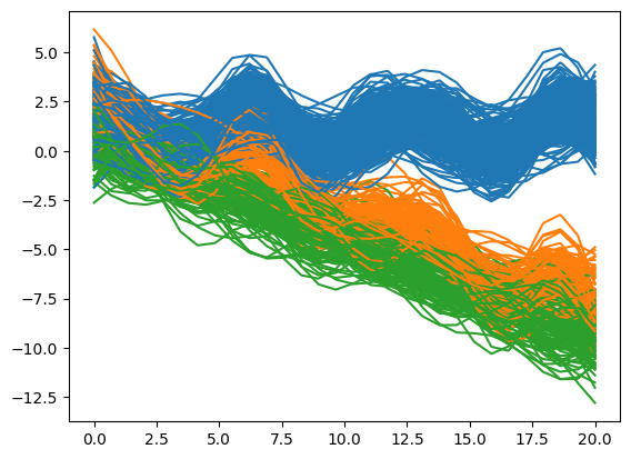
Create a Smoother object to smooth the raw data. You can specify the basis type and parameters or let the system choose automatically. Then apply fit to get the smoothed data.
Here, we use B-spline basis:
sm = Smoother(basis='bspline')
fd = sm.fit(X)
fd.plot(group=y)

Estimating the number of clusters
Use estimate_nclusters to find the optimal number of clusters by minimizing AIC or BIC:
estimate_nclusters(fd)
# Output: 3
Projection
Project the smoothed data onto chosen projection functions with Projector. Specify the projection type and number of projections. Here, we use 8 random linear combinations of leading eigenfunctions (‘rl-fpc’):
proj = Projector(basis_type='rl-fpc', n_proj=8)
coeffs = proj.fit(fd)
Ensemble Clustering: Learning GMMs and ensemble
Use UniGaussianMixtureEnsemble to cluster the data by fitting univariate GMMs to each set of projection coefficients:
Initialize with the number of clusters.
Fit GMMs using
fit_gmms.Obtain consensus clustering with
get_clustering.
We set 3 clusters as estimated earlier:
model = UniGaussianMixtureEnsemble(n_clusters=3)
model.fit_gmms(coeffs)
pred_labels = model.get_clustering()
Visualize the clustering with:
model.plot_clustering(fd)
The model also offers clustering validation metrics. For external validation, compare predicted clusters to true labels using Adjusted Mutual Information, Adjusted Rand Index, and Correct Classification Accuracy. For internal validation, use Silhouette Score and Davies-Bouldin Score on the functional data.
Calculate all metrics as follows:
model.adjusted_mutual_info_score(y)   # Adjusted Mutual Information
model.adjusted_rand_score(y)          # Adjusted Rand Index
model.correct_classification_accuracy(y)  # Correct Classification Accuracy
model.silhouette_score(fd)            # Silhouette Score
model.davies_bouldin_score(fd)        # Davies-Bouldin Score